A simple elastic behaviour

MFront implementation¶

To give a first introduction to writing material behaviors using MFront, we will implement a very simple linear elastic model :

where $\lambda$ and $\mu$ are the Lamé coefficients. The parameters of the model will be Young’s modulus $E$ and Poisson’s ration $\nu$, while the output will be the Cauchy stress tensor $\tens{\sigma}$. Of course, we could use one of Mfront’s standard brick for this purpose, but the idea here is to define everything ourselves.

Here is a look at the corresponding elasticity.mfront file:

@DSL DefaultGenericBehaviour;
@Author Maxime Pierre;
@Date 22/11/2025;

@Behaviour Elasticity;

First, we specify the domain specific language (DSL) that we want to use. It will condition what keywords we will have access to in the rest of the file. After optionally declaring an author and a date, we give a name to our behaviour (Elasticity).

Next, we define the input and output variables of our model : the strain tensor $\tens{\varepsilon}$ (a gradient of the displacement), and its associated flux which is the stress tensor $\tens{\sigma}$.

@Gradient StrainStensor εᵗᵒ;
εᵗᵒ.setGlossaryName("Strain");

@Flux StressStensor σ;
σ.setGlossaryName("Stress");

Then, we define the material properties which must be passed to the behaviour:

@MaterialProperty stress E;
E.setGlossaryName("YoungModulus");

@MaterialProperty real ν;
ν.setGlossaryName("PoissonRatio");

Now, we define the blocks composing the tangent operator. In our simple case, their is only one, $\partial\tens{\sigma}/\partial\tens{\varepsilon}$, which corresponds to the stiffness tensor $\mathbb{C}$.

@TangentOperatorBlocks{∂σ∕∂Δεᵗᵒ};
@ProvidesTangentOperator ;

Finally, we enter the core of the behaviour with the Integrator block. This is where the behaviour of the material is actually calculated. MFront provides some helper functions to calculate Lamé’s coefficients from $E$ and $\nu$. Then, we calculate the stress with an incremental formulation (note that in the case of elasticity, a total formulation would also have been acceptable). The last part gives the one tangent operator block that was declared above.

@Integrator{
  const auto λ = computeLambda(E, ν);
  const auto μ = computeMu(E, ν);
  σ += λ ⋅ trace(Δεᵗᵒ) ⋅ I₂ + 2 ⋅ μ ⋅ Δεᵗᵒ ;

  if (computeTangentOperator_) {
    ∂σ∕∂Δεᵗᵒ = λ ⋅ (I₂ ⊗ I₂) + 2 ⋅ μ ⋅ I₄;
  }
}

Compiling a behaviour¶

Once the .mfront file is written, we need to compile it to create a shared library that can then be used in other contexts (mtest, python, FEniCS...). This can be done from the terminal using the following command:

mfront --obuild --interface=generic elasticity.mfront

Here, we used the generic interface, which is the one used to plug the constitutive laws into python or FEniCS using MGIS, the MFront Generic Interface Support. The command creates or updates a shared library src/libBehaviour.so on Linux or src/libBehaviour.dylib on MacOS (note the difference in extension for dynamic libraries).

Testing the behaviour with mtest¶

@Behaviour<Generic> 'src/libBehaviour.dylib' 'Elasticity';
@MaterialProperty<constant> 'YoungModulus' 1e+10 ;
@MaterialProperty<constant> 'PoissonRatio' 0.2 ;

@ExternalStateVariable 'Temperature' 293.15 ;

@ImposedDrivingVariable 'StrainXX' 0.0;
@ImposedDrivingVariable 'StrainYY' 0.0;

@ImposedThermodynamicForce 'StressZZ' {0.0: 0.0, 1.0: -1e7};

@Times {0.0, 1.0 in 10};

mtest elasticity.mtest

Interacting with the behaviour in python¶

Using the mtest package in python, it is possible to interact with a compiled MFront behaviour.

First, we have to set the behaviour for our test as well as the different material properties that are necessary. We chose Young’s Modulus as 10 MPa and Poisson’s ration as 0.2.

Next, we set the conditions for the test. The setImposedGradient method allows to control the different components of the gradients (here strain) by their name, and the setImposedThermodynamicForce method does the same for thermodynamic forces (here stress). A single value can be provided, or a dictionary with several entries to have a variation over time, similar to the mtest syntax.

We impose oedometric conditions on the sample: $x$ and $y$ deformation are prevented while we apply an axial load up the 10 MPa in compression.

We perform a simulation with 10 steps between times 0 and 1, and store the results to show the stress-strain curve of the oedometric test. Obviously, this is a very simple test and the results is a simple line with slope $E_\mathrm{oed}$.

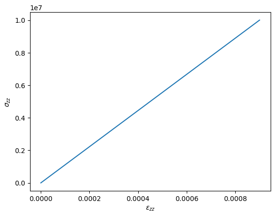
We can compare the resulting oedometric modulus from the simulation with the analytical formula: